HowTo: Activate TensorFlow automatic mixed-precision computing and execution performance analysis

This article will guide users how to use the TWSC Interactive Container step by step to train a handwritten digit recognition model on MNIST dataset with the automatic mixed precision (hereinafter referred to as AMP) enabled in TensorFlow to maintain the model accuracy and shorten the computing time. Finally, ResNet-50 is used to perform a simple performance analysis. The content outline is as follows:

• Introduction to AMP
• Create a TWSC Interactive Container
• SSH into the container
• Enable AMP
  • Environment variable setting method
  • A code example of handwritten digit recognition on MNIST dataset
• Benchmark performance analysis: ResNet-50 v1.5

Introduction to AMP

Traditional high-performance computing uses Double Precision computing to ensure the convergence of numerical algorithms (e.g., atmospheric simulation). However, Double precision computing (FP32) requires a lot of memory space since it uses 32 bits to represent 16 digits of floating point.

Some numerical computing (e.g., deep learning) does not need to rely entirely on double-precision computing. The use of automatic mixed precision computing (AMP) can speed up the computing speed and maintain the accuracy of the model.

info

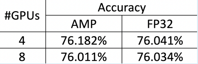
💡 The following tests shows that the accuracy of the model is indeed not affected by AMP:

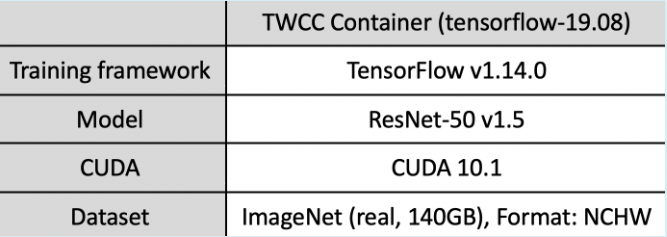
• Using ResNet-50 v1.5 model for image recognition model training on ImageNet dataset (140 GB)

• Using 4 or 8 GPUs, after 50 epochs training, the accuracy is as follows. Double precision computing (FP32) and automatic mixed precision computing (AMP) show similar accuracy:

The following tutorial demonstrates how to enable AMP in TWSC Interactive Container.

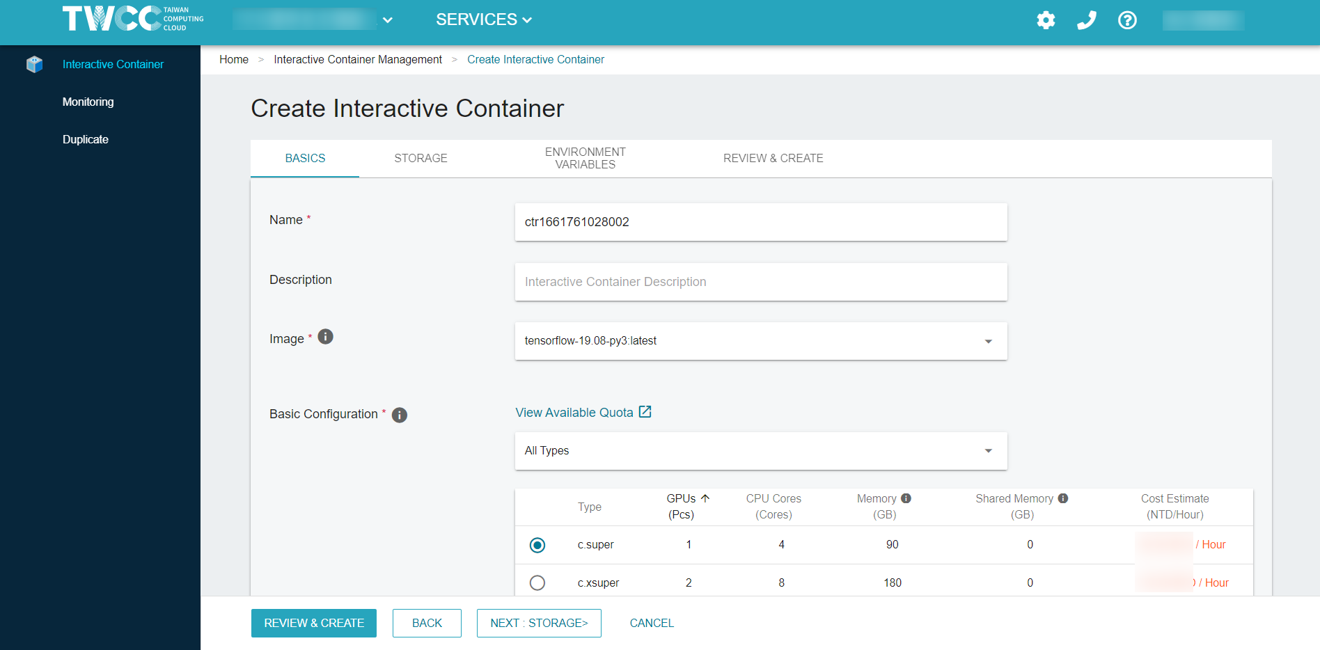
Create a TWSC Interactive Container

After signing in, please refer to Create an interactive container and create a container with following settings:

Image type          : TensorFlow
Image version       : tensorflow-19.08-py3:latest
Basic configuration : c.super

SSH into the container

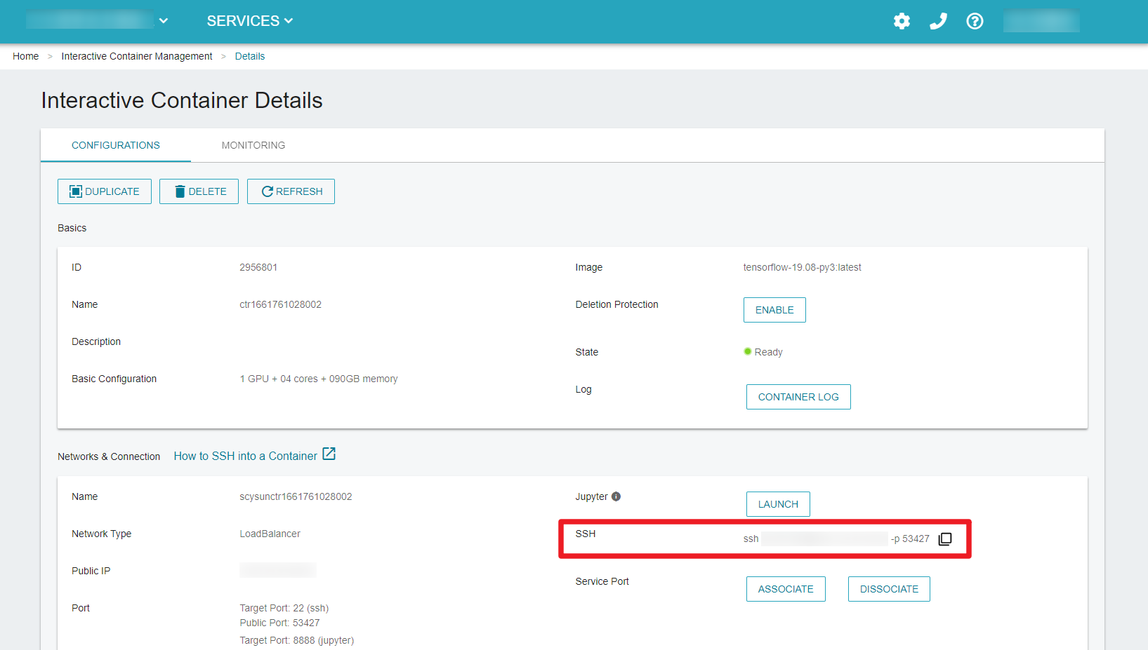
On the Interactive Container Management page, click the container to enter the Interactive Container Details page when the container state changes from Initializing to Ready. We use SSH to connect to the container in this tutorial, and Jupyter Notebook is another option. For detailed steps, please refer to Using SSH connection sign in.

Enable AMP

Enabling AMP involves two steps: setting environment variables and rewriting the computing program. The demonstration is as follows:

Environment variable setting method

To set the environment variable in the bash shell, you can directly enter the commands in the command line as follows:

export TF_ENABLE_AUTO_MIXED_PRECISION=1
export TF_ENABLE_AUTO_MIXED_PRECISION_GRAPH_REWRITE=1

info

💡 In TWSC Interactive Container (TensorFlow 19.08-p3:latest), AMP is enabled by default, you can use the command echo $TF_ENABLE_AUTO_MIXED_PRECISION to verify:
Response = 1 means AMP is enabled
Response = 0 means AMP is stopped

Code examples

• Graph-based example：

opt = tf.train.AdamOptimizer()
opt = tf.train.experimental.enable_mixed_precision_graph_rewrite(opt)
train_op = opt.miminize(loss)

• Keras-based example：

opt = tf.keras.optimizers.Adam()
opt = tf.train.experimental.enable_mixed_precision_graph_rewrite(opt)
model.compile(loss=loss, optimizer=opt)
model.fit(...)

A code example of handwritten digit recognition on MNIST dataset

In Python, AMP can be enabled in Keras with the collocation of TensorFlow to train a handwritten digit recognition on MNIST dataset as follows:

import tensorflow as tf
start_time = time.time()
opt=keras.optimizers.Adadelta()
opt = tf.train.experimental.enable_mixed_precision_graph_rewrite(opt)
model.compile(loss=keras.losses.categorical_crossentropy,
              optimizer=opt,
              metrics=['accuracy'])
elapsed_time = time.time() - start_time
print('Time for model.compile:', elapsed_time)

info

💡 The KerasMNIST.py (AMP disabled) and kerasMNIST-AMP.py (AMP enabled) program files can be downloaded here for reference.

Benchmark performance analysis: ResNet-50 v1.5

The following table shows the performance comparison of five image recognition training using ResNet-50 v1.5 with different settings:

Group	AMP	XLA	Precesion	Batch Size
1	❎	❎	Double precision	128 (Baseline)
2	❎	❎	Double precision	256
3	✅	❎	Mixed precision (single and half precision)	256
4	✅	✅	Mixed precision (single and half precision)	256
5	✅	✅	Mixed precision (single and half precision)	512

info

Accelerated Linear Algebra (XLA) can optimize TensorFlow computing and accelerate processing speed.

When you create a TWSC Interactive Container (TensorFlow 19.08-p3:latest), the sample code of ResNet-50 v1.5 already exists in the /workspace/nvidia-examples/resnet50v1.5 directory. Create a new directory (e.g., results) under this directory to store the model data. Enter the command in the command line as follows:

cd /workspace/nvidia-examples/resnet50v1.5
mkdir results

Group 1. Control group: Baseline

AMP disabled | Double precision｜Batch size = 128

The environment enables automatic mixed precision by default, so the execution control group must disable the automatic mixed precision in the environment variable in advance. To do so, directly enter the execution command in the command line as follows:

export TF_ENABLE_AUTO_MIXED_PRECISION=0
export TF_ENABLE_AUTO_MIXED_PRECISION_GRAPH_REWRITE=0
python ./main.py --mode=training_benchmark --warmup_steps 200 \
       --num_iter 500 --batch_size 128 --iter_unit batch --results_dir results \
       --nouse_tf_amp  --nouse_xla

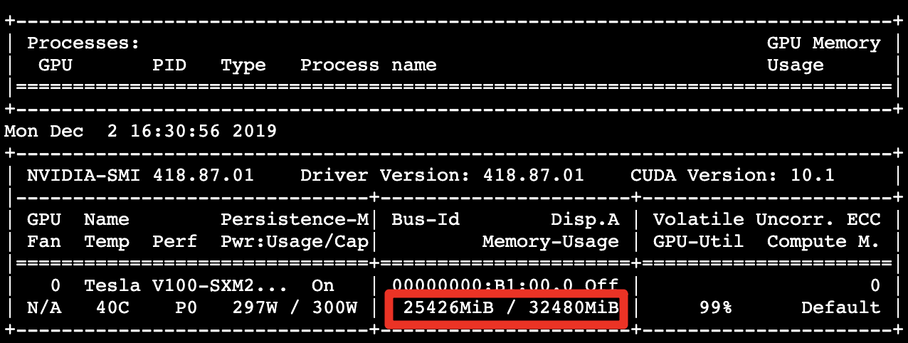
Using the following command to dynamically observe the usage of GPU memory every 10 seconds. We can observe that the GPU memory usage is about 25.43 GB. The GPU memory capacity allocated (32.48 GB) is not yet fully utilized.

nvidia-smi --loop=10

The model training completed, and it could process about 393.49 images per second:

Group 2. Batch Size 256

AMP disabled | Double precision | Batch size = 256

From the control group, we dynamically observe the usage of GPU memory and find that the GPU memory has not been fully utilized, so we doubled the batch size and directly entered the execution command in the command line as follows:

rm -rf results/*
python ./main.py --mode=training_benchmark --warmup_steps 200 \
       --num_iter 500 --batch_size 256 --iter_unit batch --results_dir results \
       --nouse_tf_amp  --nouse_xla

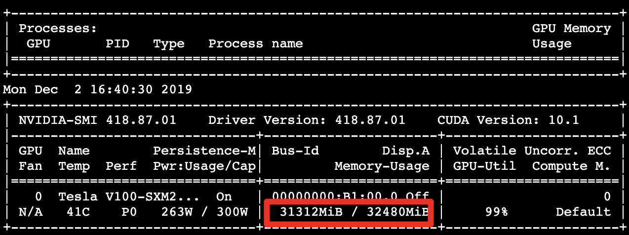
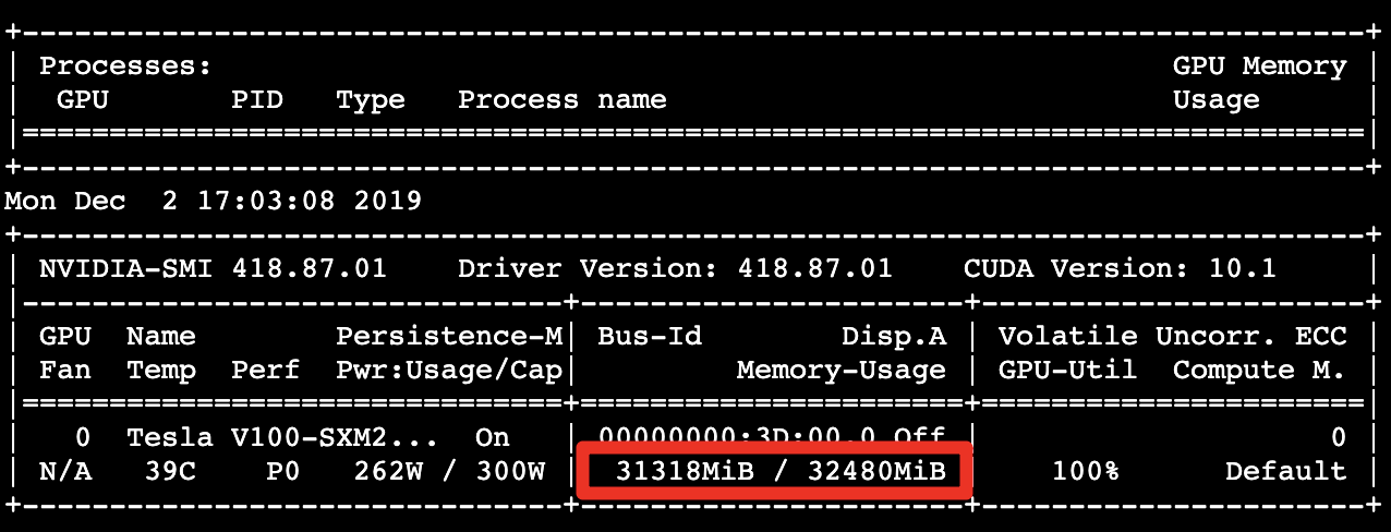
GPU memory usage: 31.31 GB

Processing about 405.73 images per second, showing performance 1.03 times better than the control group.

Group 3. AMP enabled

Enable AMP | Mixed precision (single and half precision)｜Batch size = 256

Enter the following command to set the environment variable to enable AMP, and perform computing:

rm -rf results/*
export TF_ENABLE_AUTO_MIXED_PRECISION=1
export TF_ENABLE_AUTO_MIXED_PRECISION_GRAPH_REWRITE=1

python ./main.py --mode=training_benchmark --warmup_steps 200 \
       --num_iter 500 --batch_size 256 --iter_unit batch --results_dir results \
       --nouse_xla

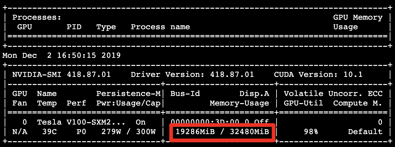
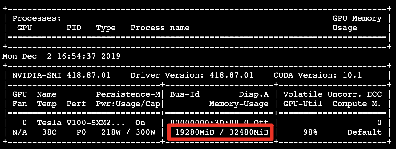
GPU memory usage has been reduced to 19.28 GB.

Processing about 1308.37 images per second, showing performance 3.33 times better than the control group.

Group 4. XLA enabled

AMP & XLA enabled | Mixed precision (single and half precision) | Batch size = 256

Enter the command directly in the command line as follows:

rm -rf results/*
python ./main.py --mode=training_benchmark --warmup_steps 200 \
       --num_iter 500 --batch_size 256 --iter_unit batch --results_dir results

GPU memory usage: 19.29 GB

Processing about 1309.21 images per second, showing performance 3.33 times better than the control group.

Group 5. Double the batch size again

AMP & XLA enabled | Mixed precision (single and half precision) ｜Batch size = 512

ResNet-50 v1.5 Benchmark performance analysis example

You can run the performance analysis of ResNet-50 directly through the following commands, the running time is about 3 minutes
wget -q -O - http://bit.ly/TWCC_CCS_AMP-XLA | bash

Since AMP greatly reduces the usage of GPU memory, we double the batch size in an attempt to increase the execution performance. Enter the command directly in the command line as follows:

rm -rf results/*
python ./main.py --mode=training_benchmark --warmup_steps 200 \
       --num_iter 500 --batch_size 512 --iter_unit batch --results_dir results

GPU memory usage: 31.31 GB

Processing about 1361.00 images per second, showing performance 3.46 times better than the control group.

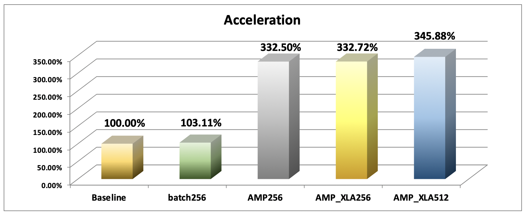
Performance comparison

Summarizing the above image processing data results (img/sec, GPU memory usage) for each group, the performance comparison is shown in the following chart. Compared with the control group, the performance of enabling AMP acceleration is quite significant in reducing GPU memory usage and shortening training computing time:

Group	AMP	XLA	Precesion	Batch Size	Number of images processed per second (img/sec)	GPU memory usage (GB)
1 (Baseline)	❎	❎	Double precision	128	393.49	25.43
2	❎	❎	Double precision	256	405.73	31.31
3	✅	❎	Mixed precision (single and half precision)	256	1308.37	19.29
4	✅	✅	Mixed precision (single and half precision)	256	1309.21	19.29
5	✅	✅	Mixed precision (single and half precision)	512	1361.00	31.31